The Evolution of LLM Inference: Decoding algorithms — Part 1

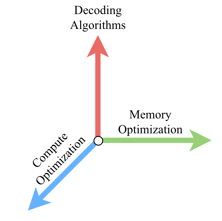
LLM inference optimization can be understood along three major axes: memory optimization, compute optimization, and decoding algorithms. Compared to memory and compute optimizations, decoding algorithms are often discussed less, even though they are becoming increasingly important for fast LLM serving. This article focuses mainly on decoding algorithms: how we moved from naive autoregressive decoding to speculative decoding, multi-head prediction, tree-based verification, draft-free speculative decoding and long-context speculative decoding. Memory and compute optimizations will also be mentioned later, because in real-world inference systems these techniques are used together.

Content:

🎯 Motivation
⚙️ Classic Speculative Decoding
🌲 Tree Speculative Decoding
🧩 Multi-head Speculative Decoding
🚀 Draft-Free Speculative Decoding (Part 2)
📖 Long-Context Speculative Decoding (Part 2)
💾 Memory and Compute Optimizations (Part 2)

🎯 Motivation

Why focus on decoding algorithms?

The early story of LLM inference was simple: give the model a prompt, run a forward pass, produce one token, append it to the context, and repeat. This naive autoregressive loop is elegant, but brutally inefficient.

Every generated token depends on the previous token, so generation becomes a long chain of sequential model calls. For a 100-token answer, the model may need around 100 decoding steps. This is the core bottleneck that nearly every modern LLM inference technique tries to attack.

The evolution of LLM inference is not just about “making transformers faster.” It is about reducing repeated work, improving GPU utilization, managing memory, predicting multiple tokens per step, and serving many users efficiently.

The first wave of LLM inference optimization made each decoding step cheaper: KV cache avoided recomputation, batching improved GPU utilization, PagedAttention managed memory, and FlashAttention and quantization made kernels faster.

But these methods still operate inside the same basic loop: generate one token, run the model again, generate the next token.

KV cache, batching, and FlashAttention made each decoding step faster. The next frontier is reducing the number of decoding steps.

The newer wave of inference research asks a deeper question:

Can we generate or verify multiple future tokens in parallel?

So the next frontier of LLM inference is not only making one step faster. It is reducing the number of decoding steps by predicting, drafting, or verifying multiple future tokens in parallel.

This article focuses mainly on these decoding algorithms that reduce the number of decoding steps.

⚙️ Classic Speculative Decoding

Overview:

What problem speculative decoding solves?

LLM generation is slow because decoding is autoregressive.

At inference time, the model generates:

token_1 → token_2 → token_3 → token_4 ...

Each new token depends on all previous tokens, so the large model usually needs one forward pass per generated token.

For a large model, this becomes expensive because every decoding step reads the model weights, updates the KV cache, computes attention, and produces logits.

Classic speculative decoding tries to reduce the number of expensive large-model forward passes.

The idea is that a smaller model can cheaply guess future tokens, while the large model verifies those guesses in parallel.

— — — — — — — — — — — — — — — — — — — — — — —

Core idea: Draft model + Target model

— — — — — — — — — — — — — — — — — — — — — — —

Classic speculative decoding uses two LLM models:

Draft model:  small, fast, cheap
Target model: large, accurate, expensive

Step 1: Draft several tokens

The draft model proposes several future tokens:

Prompt:        The capital of France is
Draft tokens:  Paris . It

Step 2: Verify using target model

Then the target model checks these tokens in one parallel forward pass.

Each draft token is compared against what the target model would have produced.

Draft:   Paris   .   It
Target:  Paris   .   The

Step 3: Accept or reject draft tokens

In greedy selection, this is simple:

Accept token if:
draft_token == target_model_argmax_token

Example:

Draft:   Paris   .   It
Target:  Paris   .   The

Then:

Paris -> accepted
.     -> accepted
It    -> rejected

The output becomes:

Paris .

Then decoding continues from there.

Step 4: Generate one correction token

When rejection happens, the target model provides the correct next token. So even when the draft fails, the target model still contributes useful progress.

Strategies to accept or reject tokens:

This dives deep into step 3 mentioned above.

Greedy vs sampling mode

Case 1: Greedy

Greedy selects the highest-probability token:

next_token = argmax(logits)

Verification is simple:

if draft_token == target_argmax_token:
    accept
else:
    reject

This is easier to implement and debug.

Case 2: Sampling

Algorithm:

1. Draft model produces logits
2. Apply temperature / top-k / top-p if enabled
3. Sample one draft token from that filtered draft distribution q
4. Target model computes probability p for that same token
5. Draw u ~ Uniform(0, 1)
6. Accept if u <= min(1, p(token) / q(token))

Sampling uses probabilities:

top-k sampling
top-p sampling
temperature sampling

Here, the draft token may not exactly match the target model’s most likely token. Instead, the algorithm compares the draft model probability and the target model probability.

A simplified acceptance rule is:

accept with probability min(1, p_target(token) / p_draft(token))

Acceptance and rejection:

accept_prob = min(1, p_target[token] / p_draft[token])
u = random number between 0 and 1
if u <= accept_prob:
    accept token
else:
    reject token

Important:

u sample random number. This is generated for each draft token for selection. This is normal rejection sampling.

If the token is rejected, the next token is sampled from a corrected distribution.

This is more complex, but it is necessary if you want speculative decoding to preserve the target model’s sampling behavior.

Let’s take an example and understand this:

**********Scenario 1: Target model likes the token more

p_target(x) > p_draft(x)

Example:

p_target("Paris") = 0.60
p_draft("Paris")  = 0.30

Then:

p_target / p_draft = 0.60 / 0.30 = 2
min(1, 2) = 1

So we accept with probability 1.

Meaning: The draft model proposed a token that the target model also strongly supports. So keep it.

**********Scenario 2: Draft model overestimated the token

p_target(x) < p_draft(x)

Example:

p_target("London") = 0.10
p_draft("London")  = 0.50

Then:

p_target / p_draft = 0.10 / 0.50 = 0.20

So we accept only with probability 0.20.

Meaning: The draft model proposed this token highly compared to the target model. So we assign low probability for final selection.

This prevents the draft model from changing the target model’s distribution.

Important point:

The draft model does not decide the final output.
The target model decides which draft tokens are valid.

The draft model is only a proposer. The target model is the verifier.

This is why speculative decoding is often called: draft-then-verify decoding or proposal-and-verification decoding

The target model verifies multiple proposed tokens in parallel, which reduces the number of serial target-model calls, resulting in reduced inference latency.

Won’t smaller draft model degrade the output quality?

To avoid output quality degradation, it is important for the draft model to match the target model’s decoding distribution.

Ideally, classic speculative decoding should be lossless with respect to the target model.

That means the final generated distribution should match the target model’s normal decoding distribution.

For greedy selection, this is easy to understand:

Only accept a token if the target model would have selected the same token. As explained above in the subsection ‘Case 1: Greedy’

For sampling,

The algorithm uses a rejection-sampling correction rule so that the final distribution still matches the target model distribution. As explained above in the subsection ‘Case 2: Sampling’

Key production parameters

1. Draft length

This is the number of tokens the draft model proposes per iteration.

Common values:

k = 2, 4, 8

Higher k gives more possible speedup, but also more wasted work if many draft tokens are rejected.

2. Draft model size

The draft model must be much faster than the target model.

Example:

Target: 70B
Draft: 7B or 1B

But the draft model must also be accurate enough. If it is too weak, the acceptance rate becomes low.

3. Acceptance rate

This is the key metric.

acceptance_rate = accepted_draft_tokens / proposed_draft_tokens

High acceptance rate means good speedup. Low acceptance rate means speculative decoding may become slower than normal decoding.

4. Tokenizer compatibility

The draft and target model should ideally use the same tokenizer.

If tokenizers differ, token alignment becomes difficult and production implementation becomes messy.

When classic speculative decoding works well ?

Classic speculative decoding works best when:

The draft model is much smaller than the target model.
The draft model predicts similar tokens to the target model.
The task has predictable continuations.
The tokenizer is shared.

Good use cases:

Code completion
Chatbot responses
Summarization
Translation
Structured generation
Repetitive formatting tasks

Why these work well:

The draft model can often guess easy next tokens correctly.
The target model only needs to verify.

When it fails or gives little speedup ?

Speculative decoding may not help when:

The draft model is too weak.
The target model is already highly optimized.
The workload has high randomness.
Temperature is high.
Top-p sampling is aggressive.
The draft and target tokenizers differ.
The accepted-token rate is low.
The draft model adds too much GPU memory pressure.

Bad cases:

Creative writing with high temperature
Very hard reasoning
Highly uncertain next-token distributions
Long-tail domain-specific text

In these cases, the draft model guesses poorly, so many tokens are rejected.

What metrics to track ?

Number of output tokens/sec
Time-to-first-token
Inter-token latency
Acceptance rate
GPU memory usage
Draft overhead
Target forward-pass count

These metrics are also applicable to all the other speculative decoding algorithms.

🌲 Tree Speculative Decoding

Overview:

Tree speculative decoding is an extension of speculative decoding where the draft stage proposes a tree of possible future tokens instead of a single sequence. The target LLM then verifies many candidate paths in one forward pass using tree attention, where each candidate token attends only to its own ancestors. This increases the chance of accepting multiple tokens per target-model call, especially when the draft model is uncertain among several plausible continuations.

Why use Tree speculative decoding?

Classic speculative decoding asks a small draft model to propose multiple future tokens, then the large target model verifies them in parallel. But classic speculative decoding usually proposes one linear chain of tokens:

A → B → C → D

Problem: if token B is wrong, then C and D are also discarded.

Tree speculative decoding solves this by proposing multiple possible branches:

          A
       /  |  \
      B   C   D
     / \  |   / \
    E  F  G  H  I

Instead of betting on one draft sequence, it verifies many candidate draft sequences in one target-model pass.

Core Idea of Tree Speculative Decoding

Tree speculative decoding replaces a single draft path with a draft tree.

Instead of:

the → cat → sat → down

the draft model proposes:

              the
        /      |      \
      cat     dog     man
     /  \      |       |
   sat  ran   barked  walked

Each node is a candidate token. Each root-to-node path is a possible continuation. The large model then verifies all tree nodes in one forward pass using a special attention mask called tree attention.

Token Tree Construction

The first major design problem is: how do we build the tree?

There are multiple ways.

Method 1: From a small draft model

A small draft model generates top candidates at each step.

Example:

Step 1 top-3:
["cat", "dog", "man"]
For "cat", next top-2:
["sat", "ran"]
For "dog", next top-2:
["barked", "slept"]

This creates:

          prompt
       /    |    \
    cat    dog   man
   /  \    /  \
sat  ran barked slept

Implementation-wise, these branch expansions can be batched per tree level.

So tree construction is:

Level 1: one draft forward pass
Level 2: batched draft forward pass over all level-1 branches
Level 3: batched draft forward pass over all level-2 branches

Therefore, tree construction is still sequential across depth, but parallel across branches at the same depth.

This helps to compute multiple sequences faster.

Method 2:

This method uses multi-head multi-token prediction draft models. This will be covered in next sections clearly. Mentioning here for completion.

Tree Attention

This is the most important part.

In normal causal attention, token i can attend to all previous tokens:

token_4 attends to: token_1, token_2, token_3

But in a tree, during draft verification, a node should attend only to:

prompt tokens + its ancestor nodes

Example tree:

          prompt
          /    \
        A       B
       / \      |
      C   D     E

For node D, the valid context is:

prompt + A + D

It should not attend to B, C, or E.

So we need a tree attention mask.

The mask says:

A can attend to prompt
B can attend to prompt
C can attend to prompt + A
D can attend to prompt + A
E can attend to prompt + B

This tree attention mask is provided to target model during draft verification process, in order to verify all the sequence in parallel in one single forward pass.

Token Acceptance Logic

Draft model creates tree

Example tree:

Prompt: "The cat"

                 root
              /        \
            sat         ran
          /    \       /   \
        on    near   away  fast
       /  \
     the   a

Flatten the tree:

tree_tokens = [sat, ran, on, near, away, fast, the, a]

Target model gets all tree tokens at once. The input to target model is conceptually:

Prompt + [sat, ran, on, near, away, fast, the, a]

But because of tree attention mask, each token sees only its valid path.

The target model outputs logits for every tree position (for every token in each sequence) in one single forward pass.

So the target model computes:

P_target(sat | Prompt)
P_target(ran | Prompt)
P_target(on   | Prompt + sat)
P_target(near | Prompt + sat)
P_target(away | Prompt + ran)
P_target(fast | Prompt + ran)
P_target(the | Prompt + sat + on)
P_target(a   | Prompt + sat + on)

All of this is available after one forward pass.

After the forward pass, we have target probabilities for every candidate edge in the tree.

Now selection is just a tree traversal over already-computed probabilities.

Two selection methods: 1. Greedy selection, 2. Sampling selection

For greedy selection:

At root, choose highest target-prob child:
sat = 0.70 > ran = 0.20
choose sat

Now move to sat.

From sat:
on = 0.60 > near = 0.25
choose on

Now move to on.

From on:
the = 0.55 > a = 0.35
choose the

Final selected path:

sat → on → the

Output appended:

"The cat sat on the"

For sampling:

We do not choose max. We sample using target probabilities.

Already computed:

From root:
sat = 0.70
ran = 0.20
other = 0.10

Suppose sampling selects:

sat

The selection code is following (similar to sampling selection in classic speculative decoding):

accept_prob = min(1, p_target[token] / p_draft[token])
u = random number between 0 and 1
if u <= accept_prob:
    accept token
else:
    reject token

Then use already-computed probabilities from the sat node:

From sat:
on = 0.60
near = 0.25
other = 0.15

Suppose sampling selects:

on

Then use already-computed probabilities from the on node:

From on:
the = 0.55
a = 0.35
other = 0.10

Suppose sampling selects:

the

Final selected path:

sat → on → the

Production Design Choices

1. Tree width: Width means number of candidates per level. Higher width gives better chance of acceptance but increases verification cost.
2. Tree depth: Depth means how many future positions are drafted. Too deep can waste compute because later tokens are less likely to be accepted.
3. Static tree vs dynamic tree

Static tree:

Always use same width and depth.

Dynamic tree:

Use larger tree when draft confidence is high.
Use smaller tree when uncertainty is high.

4. Single-user latency vs batch throughput: Speculation usually improves single-request latency. But in high-throughput serving, large trees can increase GPU work and hurt batching efficiency.

When Tree Speculative Decoding Helps?

It helps when:

1. Draft model is cheap
2. Draft predictions are accurate
3. Target model is large
4. Batch size is not already saturating GPU
5. Acceptance length is high

It helps less when:

1. Draft model is weak
2. Sampling temperature is high
3. Outputs are highly uncertain
4. Batch serving is already GPU-saturated
5. Tree verification overhead is large

🧩 Multi-head Speculative Decoding

Why?

Multi-head speculative decoding is needed because standard LLM decoding predicts only one token per forward pass, making generation slow and sequential. By adding multiple lightweight heads, the model can predict several future tokens at once and verify them in parallel, reducing decoding steps.

Two popular methods for multi-head prediction are Medusa and Hydra. Both try to reduce the number of expensive large-model decoding steps by predicting multiple future tokens at once using the target LLM itself, instead of using a separate draft model.

1. Medusa adds multiple lightweight, independent prediction heads to the base LLM, where each head predicts a future token position.
2. Hydra improves medusa idea by using dependent heads, where later heads are conditioned on earlier drafted tokens, making the generated token paths more coherent.

Medusa and Hydra are draft-model-free speculative decoding techniques because they do not require a separate small draft LLM.

The same target LLM is extended with extra heads to generate and verify draft tokens.

Overview:

MEDUSA: multi-head speculative decoding

Medusa adds extra small heads on top of the base LLM. These heads are trained to produce future tokens.

IMPORTANT:

Medusa does not need a separate draft model like classic speculative decoding.

MEDUSA and HYDRA are Draft-model-free speculative decoding techniques.

Draft-model-free speculative decoding means no separate draft LLM. Target LLM and Draft LLM are same.

This makes deployment simpler because you do not need to maintain a separate small model.

Step 1 and 2: Draft tokens and Tree creation:

Medusa creates the tree draft using multiple prediction heads attached to the LLM. It does not use a separate draft model.

Each head gives top-k candidates, not just one token. So Medusa combines these candidates into a tree of possible continuations.

Suppose Medusa has 3 heads. At the current position, each head predicts future tokens:

Head 1 predicts next token candidates:
A, B
Head 2 predicts second-token candidates:
C, D
Head 3 predicts third-token candidates:
E, F

A simple tree could be:

          root
        /      \
       A        B
     /  \      /  \
    C    D    C    D
   / \  / \  / \  / \
  E  F E  F E  F E  F

Each path is one possible draft sequence:

A C E
A C F
A D E
A D F
B C E
B C F
B D E
B D F

Step 3: Verification

The base LLM receives all candidate tree nodes and a special tree attention mask.

The tree attention mask ensures each candidate token only attends to its valid ancestors.

Example:

root
 ├── A
 │    ├── C
 │    │    └── E
 │    └── D
 └── B
      └── C

Token E under path A → C → E can attend to:

context + A + C

But it cannot attend to unrelated branches like:

B or D

The LLM does one forward pass to verify many branches in parallel while preserving autoregressive correctness using the tree attention mask.

Step 4: Final token sequence selection

After the verification pass, Medusa has probabilities for every tree node. Now it does not accept all good branches. It chooses one path from the tree. The selected path is usually the longest valid path.

This is exactly similar to the Tree speculative decoding. A simple tree traversal over already-computed probabilities. It uses either greedy or sampling methods to select tokens.

HYDRA: multi-head speculative decoding

Similar to MEDUSA, except that the heads are dependent on each other. These heads are trained to produce future tokens.

Step 1 and 2: Draft tokens and Tree creation:

For Hydra, the model predictions look like this:

Head 1 predicts:
A, B
Head 2 conditioned on A predicts:
C, D
Head 2 conditioned on B predicts:
G, H
Head 3 conditioned on A-C predicts:
E, F
Head 3 conditioned on A-D predicts:
I, J
Head 3 conditioned on B-G predicts:
K, L
Head 3 conditioned on B-H predicts:
M, N

So the Hydra tree becomes:

              root
            /      \
           A        B
         /  \      /  \
        C    D    G    H
       / \  / \  / \  / \
      E  F I  J K  L M  N

The key difference:

Medusa:
same second-level candidates reused across branches

Hydra:
second-level candidates depend on the first token in that branch

Hydra draft-tree creation is sequential across heads, but parallel/batched within each head.

Depth 1:
Head 1 runs once on root
→ outputs A, B
Depth 2:
Head 2 waits for A, B
Then runs on batch [A, B]
→ outputs children for A and children for B
Depth 3:
Head 3 waits for depth-2 branches
Then runs on batch [A-C, A-D, B-G, B-H]
→ outputs children for each branch

Hydra is more accurate than Medusa, but also slightly more draft-costly.

Step 3: Verification

Now the full tree is sent to the base LLM in one forward pass using a tree attention mask.

Important:

The base model does not see all tree tokens as one normal sequence. It sees each node only with its own ancestors.

So the tree attention mask makes many branches look like many separate candidate continuations, but packed into one forward pass.

Step 4: Final token sequence selection

After the base model verifies the tree, it gives probability distributions for every node. Now Hydra compares the draft tokens against what the base model would accept. Similar to the Tree Speculative decoding and Medusa, HYDRA uses tree-traversal, and greedy or sampling methods for the final token sequence selection.

When to use Medusa or Hydra (Multi-head speculative decoding):

Use Medusa/Hydra when:

You serve an LLM interactively
You care about token latency
You want acceleration without a separate draft model
You can modify and train the model
You can use custom decoding kernels/code

Avoid them when:

You cannot fine-tune or modify the model
Your workload is already large-batch throughput optimized
Your sampling temperature is very high
Your serving framework does not support tree verification

The Part-2 of this article will cover next topics:

🚀 Draft-Free Speculative Decoding (Part 2)
📖 Long-Context Speculative Decoding (Part 2)
💾 Memory and Compute Optimizations (Part 2)

(Coming out soon …..)